Graph spanners are important for graph applications where we want to reduce the number of edges in a graph without affecting the navigability of the graph.
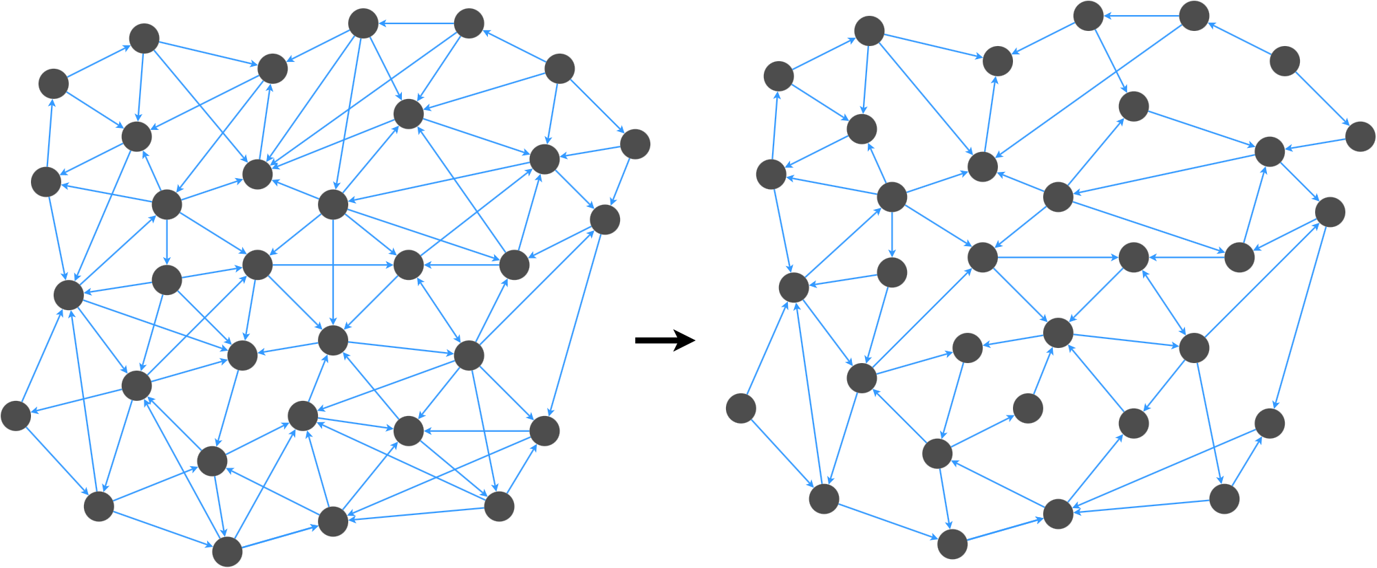
We want to remove edges while preserving important properties of the graph.
What is a Graph Spanner
Given an input graph \(G = (V,E)\), a graph spanner is a subgraph \(G_s \subseteq G\) with the k-spanner property.
Definition 1: K-Spanner Property For all edges \((u,v) \in G\), the spanner graph \(G_s\) contains a path between \(u\) and \(v\) of length no greater than \(k\).
Note that a k-spanner preserves all distances in the graph, up to a multiplicative factor. Each edge in the original graph has a detour in the spanner of length \(\leq k\), so the overall length can only increase by a multiplicative factor of \(\leq k\).
Super Sparse Spanners: The goal of spanner research is to delete as many edges as possible from \(G\) while still preserving this property. This is NP-hard (even if you are working with special, structured graphs), so people use various heuristics to approximate the optimal solution. Most papers focus on algorithms that are classically efficient - that is, polynomial algorithms. Sadly, this does not immediately translate to an effective practical algorithm. Many of these methods are of high-degree polynomial complexity, such as \(O(N^3)\).
As a result, certain parts of spanner algorithms are not actually implementable for large-scale practical problems. Fortunately, it turns out most of the basic ideas are both classically and practically efficient. In this post, we’ll extract out the basic ideas from theoretical algorithms for directed graph spanners and discuss how to make these methods practical.
Combo Graphs
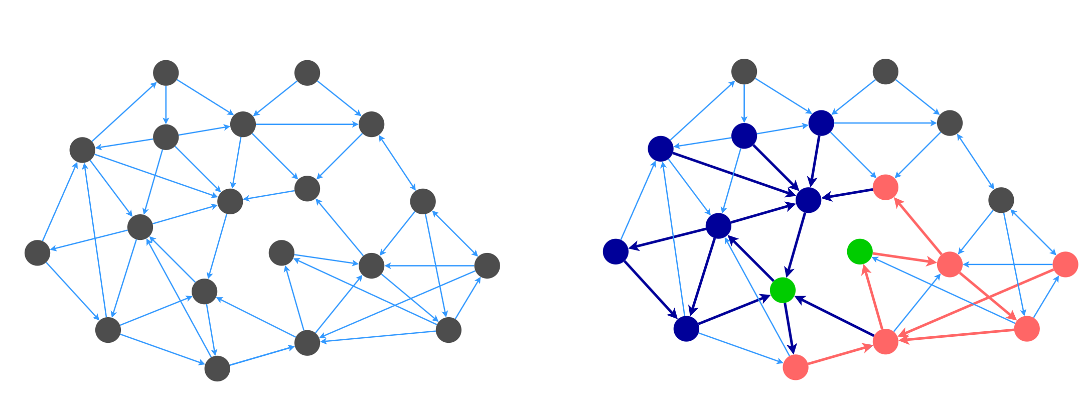
I call the first kind of directed graph spanner a combo graph. The idea is to break \(G\) into two sets of edges, and to compute a spanner for each set. Then, we combine the spanners to obtain a spanner for the overall graph.
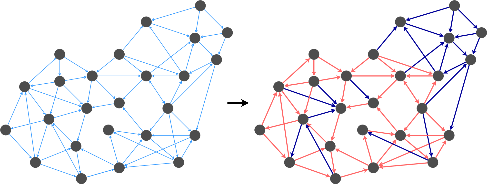
For example, we could break this graph’s edges into the red group and the dark blue group based on some decision criterion (we’ll describe this later). Once we satisfy the k-spanner property for the edges in each group, we merge the graphs back together.
Pruning: Thick and Thin
There are several spanners based on combo graphs in the literature [1-3]. Most of these algorithms rely on the idea of thick and thin edges. The thick and thin edges form the two groups that we talked about in the previous section.
Definition 2: Thick Edge Let \((V_{st},E_{st})\) be the subgraph of all paths between nodes \(s\) and \(t\) of length \(\leq k\). The edge \((s,t)\) is a thick edge if \(\|V_{st}\|\geq N/\beta\) (otherwise, it’s a thin edge).
What does Thickness Mean? A thick edge has lots of detours through the graph. The intuition is that thick edges are easier to cover because we have many alternative paths of length \(\leq k\).
Testing for Thickness: To determine whether an edge is thick or thin, we can use depth-first search to find all paths of length \(\leq k\) from \(s\). Some of these paths will connect \(s\) and \(t\). We can find \(\|V_{st}\|\) by counting the number of nodes involved in these paths.
Here is an implementation using networkx in Python.
import networkx as nx

def measure_thickness(G,s,t,k):
	# G = networkx DiGraph
	# s,t = nodes
	# k = max path length
	# returns |V_(s,t)| (subgraph induced by paths of length <= k)
	paths = nx.all_simple_paths(G, s, t, cutoff = k)
	# Note: all_simple_paths does not include any looping paths.
	# The definition from [1] technically does include looping paths
	# So this is an underestimate of the thickness
	V = set()
	for path in paths:
		for node in path:
			V.add(node)
	return len(V)

# Example for k=2 spanner
G = nx.DiGraph()
G = nx.random_k_out_graph(10, 4, 1.0, self_loops=False)
G.add_edge(0,1) # ensure that edge exists
V_01 = measure_thickness(G,0,1,2)
To implement the algorithms from [1-3], we need to check the thickness of all the edges in the graph. I suspect that this can be done using a small number of breadth-first walks through the graph rather than a depth-first search for every edge.
Pruning the Thick Edges
To get a spanner for thick edges, we use a random sampling algorithm that does the following:
- Select a random node \(v\) from the graph
- Grow a shortest-path tree (in-arborescence) from the in-connections of \(v\)
- Grow a shortest-path tree (out-arborescence) from the out-connections of \(v\)
- Add the in-arborescence and out-arborescence to the spanner
- Repeat this process \(\beta \log N\) times
- Check whether the k-spanner condition has been satisfied for all thick edges. If not, add edges until it is.
In Python, this might look like the following pseudocode.
# Et is a list of all thick edges in G, i.e. tuples (u,v)
Es = set() # spanner edges
n_iterations = int( beta * log(N) )

for i in range(n_iterations):
	v = random.choice(G.nodes())
	Tv_in = in_arborescence(G,v)
	Tv_out = out_aborescence(G,v)
	Es = Es.union(Tv_in)
	Es = Es.union(Tv_out)

for u,v in Et:
	if not is_covered(Es, u, v):
		Es.add( (u,v) )
What’s an arborescence? An arborescence rooted at \(v\) is a tree that contains a unique directed path from \(v\) to every reachable node in the graph. Minimal-cost arborescences can be found using Edmond’s branching algorithm.
How do we check coverage? We can check coverage for an edge \((u,v)\) by finding the shortest path between \(u\) and \(v\) in the spanner. This can be done efficiently by running breadth-first search in the spanner and terminating after \(k\) iterations.
Pruning the Thin Edges
There are two steps to pruning the set of thin edges. First, we solve a linear programming problem to get a set of probabilities \(x_e\) - one for each edge in the graph. Then, we sample edges according to these probabilities. Our task is to minimize the expected number of edges (i.e. the sum of \(x_e\) values) while obeying the constraints imposed by the k-spanner condition.
The deterministic version of the problem constrains \(x_e\) to the set \(\{0,1\}\), resulting in an NP-hard combinatoric optimization problem. To get around this, the authors of [1-3] relax the constraint to \(x_e \geq 0\), yielding a linear programming problem.
\[\mathrm{argmin} \sum_{e \in E} x_e\] \[\text{Subject to } \ge \|E\| \text{ constraints}\]See [1-3] for details about the constraints. Once we have the (possibly fractional) values of \(x_e\), we use randomized rounding. That is, we include an edge \(e\) in the spanner with probability proportional to \(x_e\).
def randomized_rounding(x, G):
	# x is the set of probabilities found via LP, indexed like a dictionary (s,t)->value
	# G is a networkx DiGraph
	# returns set of edges
	N = G.number_of_nodes()
	Es = [] # set of edges in spanner
	for s,t in G.edges():
		prob = x[(s,t)] * sqrt(N) * log(N)
		if (random.uniform(0, 1) < prob):
			Es.append((s,t))
	return Es
The algorithms in [1] and [2] use one version of the linear programming formulation, while the one in [3] uses a different linear program. There are also different linear programs for weighted and unweighted graphs. But at the end of the day, the algorithms all solve a highly-constrained linear program and sample edges based on the results.
Since the randomized rounding program might fail to cover all the thin edges, we have to check that all the thin edges are covered (just like we did for the thick edges).
Combining the Graphs
Once we have the two edge sets, we simply merge them to obtain the final spanner. Although it seems like the union of the two sets could contain most of the edges in the graph, the theoretical results in [1-3] show that the spanner should actually be pretty sparse.
Implementation Notes
This algorithm has several good features. It is a clever idea to satisfy the k-spanner condition for “easy” and “hard” edges separately. However, there is one big practical issue:
Linear Programming is Hard: The linear programming problem is too hard to solve for large graphs, because there will be millions of variables and inequality constraints. This is intractable even for modern solvers on high-end hardware. How can we get around this?
Don’t do Linear Programming: Fortunately, we might be able to escape the linear programming problem. For sufficiently large values of \(k\), the set of thin edges could be very small. This is especially true for “well-behaved” and navigable graphs, where most of the nodes will participate in paths that span the majority of the graph (i.e. have \(\|V_{st}\|\geq N/\beta\)). As a result, it may be possible to simply include all the thin edges without seriously inflating the number of edges in the final spanner.
Have Lots of Thick Edges: The \(\beta\) parameter controls how many edges are classified as thick, and it also decides the number of arborescences that we randomly sample. It is tempting to set \(\beta = O(N)\), so that all of the edges are thick edges. Sadly, the worst-case expected number of edges in the spanner is a factor of \(\beta\) worse than the minimal number of edges, so this could lead to bad behavior on pathological inputs.
A Practical Algorithm: I suspect that it is sufficient to run the random sampling algorithm a fixed (small) number of times, then manually add the uncovered thick edges and thin edges. While this algorithm does not preserve the worst-case theoretical guarantees for the number of edges in the spanner, it seems reasonable that it will perform well on well-behaved graphs.
Star-Spangled Spanners
The second type of graph spanner uses a generalization of star graphs to construct the spanner. In an undirected graph, a star is a set of the nodes and edges connected to a root.

For directed graphs, stars are a little more complicated - there is a tree of in-connections and a tree of out-connections. For example, here is a 2-star:
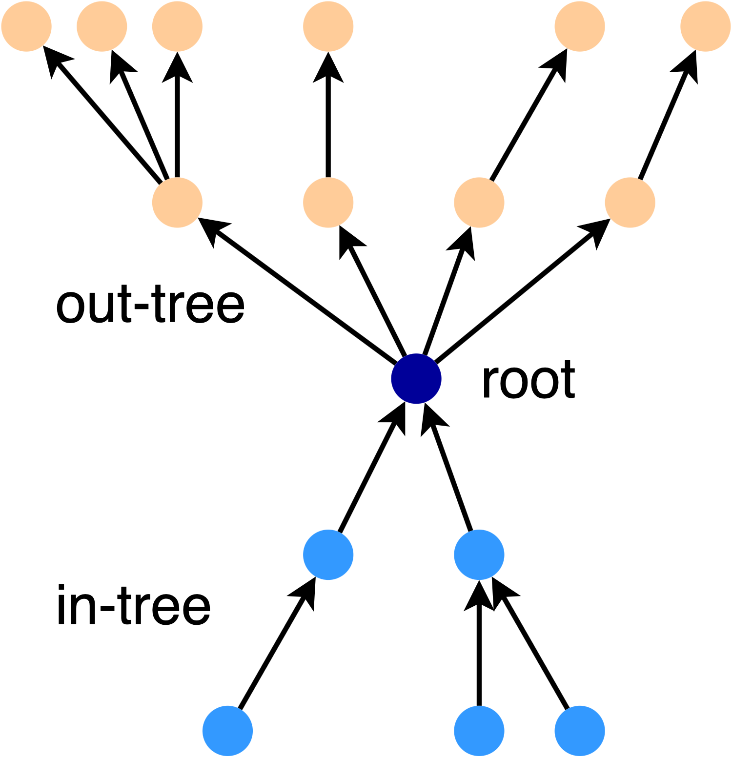
We say that an edge is covered by the star if the star graph satisfies the k-spanner condition for that edge. The key insight in [4] is that we can use a set of star graphs to cover all the edges in a graph. The final spanner can be found by intersecting the set of stars.
To see how this works, observe that the following star could cover any of the red edges between nodes (for a k-spanner with \(k = 4\)). If we include this star in the spanner, we don’t need to include any of the red edges (unless they’re part of another star in the spanner). This is because the star contains an alternative path of length \(k \leq 4\) for all of the red edges.
In general, a \(\frac{k}{2}\)-star will cover any edge from a node in the in-tree to a node in the out-tree.
Covering the Graph with Stars
The idea behind the algorithm is to sample a set of stars that cover the whole graph, while minimizing the number of edges. For example, here is a graph that is partially covered by two stars that are rooted at the green nodes.
The algorithm from [4] is as follows:
- Find the stars associated with each node in the graph.
- Find the set of edges covered by each star with a path of length \(\leq k\).
- Pick a minimal cost set of stars that cover the entire graph.
Practical Issues: The paper considers all stars with \(\leq \frac{k}{2}\) layers in the in-tree and out-tree in Step 1. This means that each node is the root of many, many stars - far too many to explicitly enumerate in a computer. Also, Step 3 is an NP-hard problem known as weighted set-cover.
Greedy Weighted Set Cover
Each star has a cost and a coverage score. The cost of a star is the number of new edges added by the star to the spanner, and the score is the number of new uncovered edges covered by the star. A standard greedy algorithm for weighted set cover is:
- Compute the costs and scores for all the choices
- Sort the choices by the relative cost ratio (cost / score) and pick the best option
- Iterate until the set is covered
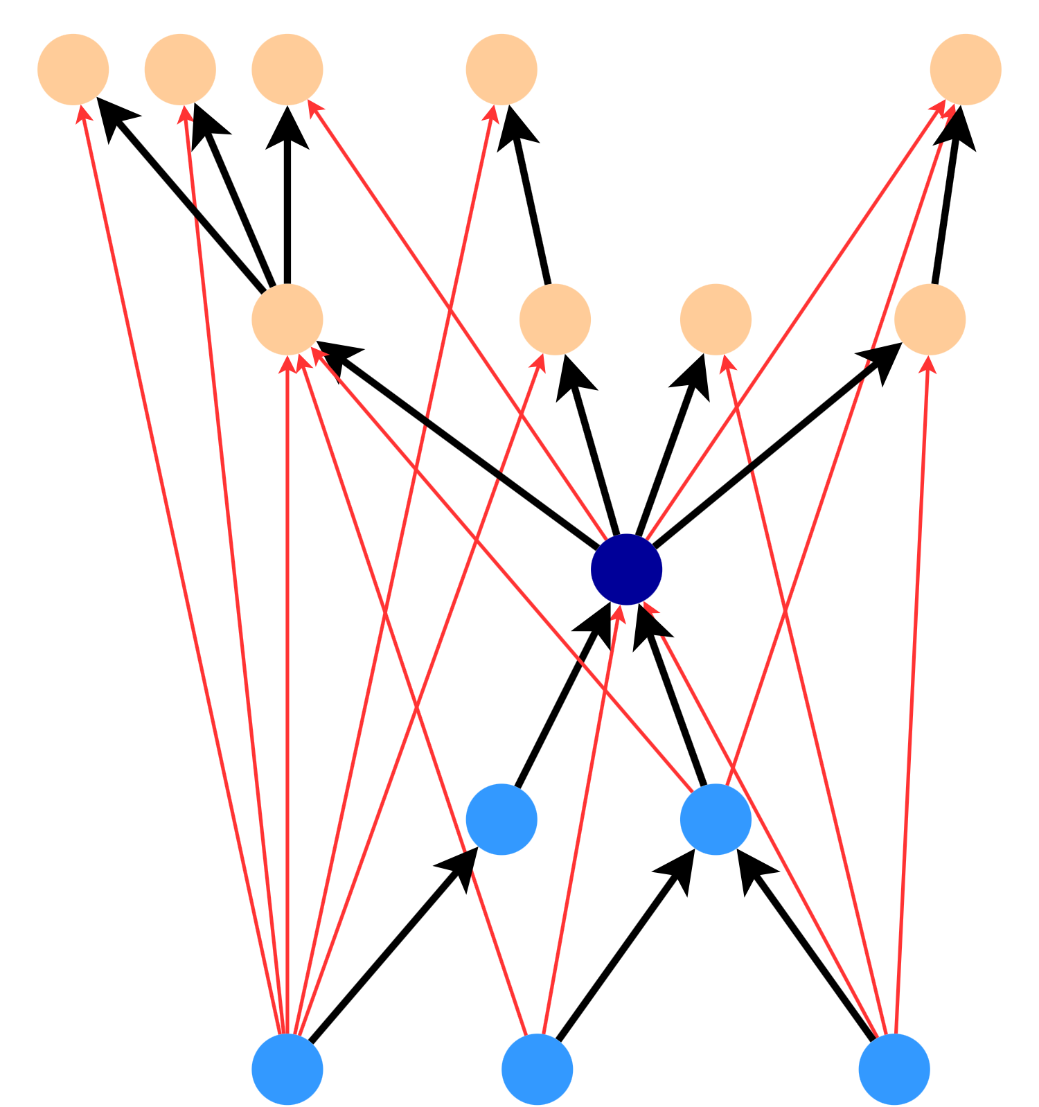
The problem is that we cannot enumerate all of the choices, because each node \(v\) provides a ton of choices - all stars around \(v\) with \(\leq \frac{k}{2}\) layers. The authors of [4] propose a workaround: construct a good star for each node \(v\), then do the greedy selection from the resulting set of \(N\) choices.
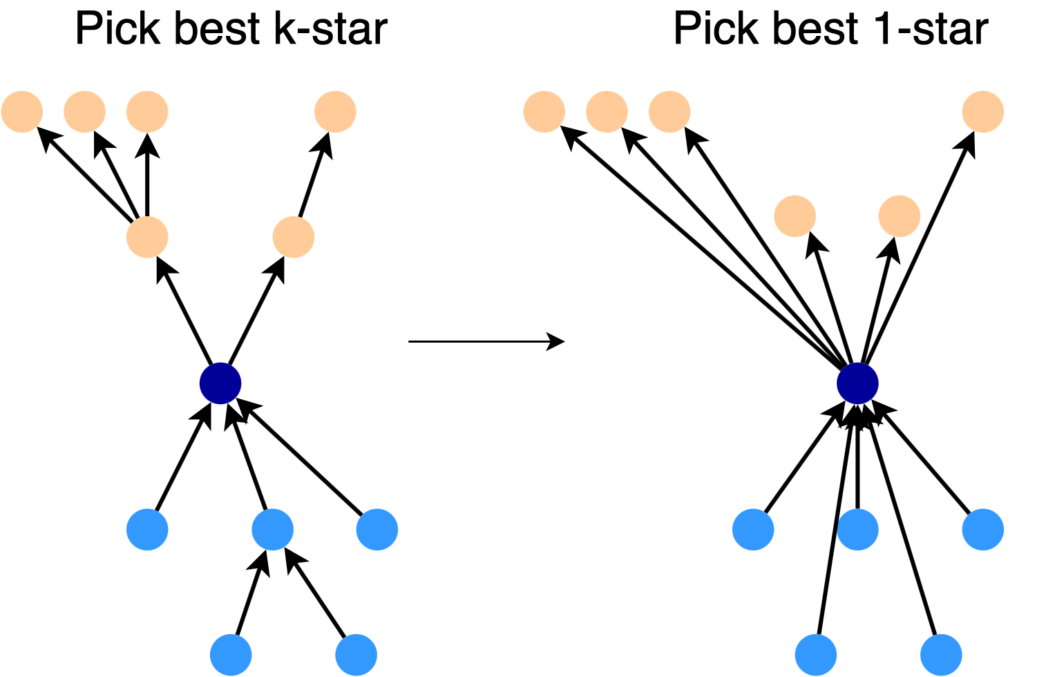
Making a Star: To construct a good \(\frac{k}{2}\)-star for a given node, we start with the full \(\frac{k}{2}\)-star. We turn this star into a 1-star by directly connecting the root to each node, as shown in the picture. Then, we pick the best subset of links in the 1-star, expand each of these links, and use the result as our \(\frac{k}{2}\)-star.
Practical Algorithm for Directed Spanners
Both the combo graphs and the star-spangled spanner are using the same fundamental idea: cover the graph using tree-like structures. The combo graphs cover the thick edges using a random set of minimal arborescences. The star-spangled spanner covers the graph using a greedy set cover of stars.
Based on these results, I think that the best practical algorithm to construct a directed spanner is some variation of the following method:
- Build an in-tree and out-tree for each node, to a depth of \(\frac{k}{2}\) layers
- [Optional] Refine the trees according to the star selection heuristic from [4]
- Score and rank all of the options by relative cost
- Pick a set of stars, either through uniform random choice, biased cost-based random selection, or a greedy algorithm
- Check that all edges are covered (add any that aren’t)
References
[1] “Improved Approximation for the Directed Spanner Problem” (ICALP 2011)
[2] “Approximation Algorithms for Spanner Problems and Directed Steiner Forest” (Elsevier Information and Computation 2013)
[3] “Directed Spanners via Flow-Based Linear Programs” (STOC 2011)
[4] “Finding Sparser Directed Spanners” (FSTTCS 2010)