At the time of writing, the most highly visited article on my website is about magnetic nanoparticles. This is funny because I haven’t touched anything stronger than a refrigerator magnet in nearly six years (I work in machine learning / AI). But I still get tons of questions about magnets - mostly from applied scientists who want to build a simluation that models their lab experiments.
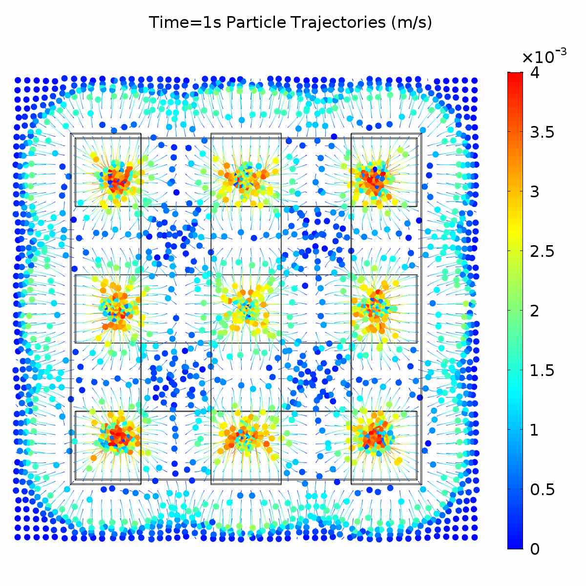
Even though I don’t work in a lab-based field anymore, I still really like computational methods and simluation. Magnetic particles are particularly cool because researchers continue to discover neat things about how they behave. For example, a recent Nature Communications paper showed that it’s possible to create interference patterns in the magnetic field strength / direction using strips of permanent magnets. I found out about this when Lingxiang Jiang reached out to me from South China University of Technology - their group wanted to model the forces exerted by these interference patterns on magnetic fluids (which somehow led them to my old blog post). We ended up collaborating on the simulation model, and the results are actually beautiful.
I’ve also had emails from folks working on drug delivery, particle filtering, energy research, computational chemistry, and more. It’s extremely gratifying to know that my work has been helpful to so many people. But I’ve noticed some common threads in the questions, and this is kind of my fault. I didn’t fully describe the details in my original blog post or even in our research papers.
Here’s a more complete guide.
Note: If you haven’t read the original post, you may want to read it beforehand. There are also some cool plots in there.
Limitations of the model
Our model makes a couple of critical assumptions. If you plan to build off of our simulation, please be aware of the following things.
Ideal point masses
First, our model operates under the assumption that the particles are ideal point masses. This is required to use the simplified expression for the force on a particle - otherwise, we’d have to consider a complicated expression that exerts different forces on different parts of the magnetic material. This assumption is reasonable for small particles, which are usually modeled as single magnetic moments, but it’s a bad approximation for large ones.
Fast magnetic response
Next, our time-dependent simulations implicitly assume that the magnetic moment of each particle is completely aligned with the applied magnetic field, and that this is true at every time step of the simulation. This assumption is reasonable as long as we’re dealing with superparamagnetic particles that have a sufficiently fast response rate when compared to the rate at which the magnetic field changes. But we can break this assumption in a couple of ways.
The first way is for the magnetic field strength or direction to change very rapidly over a small distance. As the particle moves through such a region, its magnetic moment may not have time to align with the applied magnetic field in the particle’s new location. Because the internal magnetic moment might not quite align with the applied field, the real trajectory could be slightly different than the one predicted by our model. This is also the reason why our simulations don’t work for ferromagnetic particles. These particles have a strong remnant magnetic field that persists even after we turn off or rotate the applied magnetic field. This violates our assumption because again, the magnetic moment is not necessarily in the same direction as the applied field.
The other way to break the assumption is to apply a very fast-changing magnetic field. If the applied magnetic field switches direction before the particles can orient themselves, they will experience much different forces than predicted by our simulation.
The “fast response” asssumption also has implications about the temperature of our system, because the response time of a superparamagnetic material is strongly temperature-dependent. If our particles are too cold, they will have a sluggish magnetic response and be unable to quickly orient themselves in the direction of the applied magnetic field. The so-called blocking temperature (below which there will be almost no response at all) is pretty low for the materials encountered in applications, and the sluggish response only occurs in a narrow range around this temperature. So this is not usually a problem in lab experiments conducted at room temperature, but it’s an important limitation to keep in mind if it applies to your system.
Magnetic response does not saturate
Finally, we assume that the magnetic fields are relatively small because we use a linear model of the magnetic moment. If we were to apply a really strong field - one large enough to completely saturate the superparamagnetic response - then our simluation will over-predict the strength of the force because it does not model saturation effects. This is easy to fix (e.g., by using an empirical B-H curve instead of a linear approximation), but it adds complexity to the model.
Computing magnetic forces
COMSOL has a particle tracing module, and the module has support for charged particle interactions. Unfortunately, it doesn’t have out-of-the-box support for magnetic particle interactions. It does, however, allow you to apply a user-specified force to the particles.
Our simulation approach is to calculate this force “manually.” Then, we can apply it to the particles to trace their trajectories using the particle tracing module (which is a pretty thin wrapper over the basic kinematics equations). To do this, we need to compute the force that would be applied to a particle at every location in the geometry. Fortunately, the research community has developed (and validated) a good mathematical model for the force on a superparamagnetic bead in a magnetic field.
\[\mathbf{F} = \frac{V \Delta \mathcal{X}_v}{\mu_0} (\mathbf{B} \cdot \nabla)\mathbf{B}\]In order to use this equation, we need to know the particle volume, the magnetic susceptibility, and the magnetic field. In COMSOL, we can get the magnetic field by running a stationary study of the magnetic field. My previous blog post goes into detail about how to get the B field once you have a model of the magnet.
However, it’s a little tricky to model the particles and the magnet itself. Of course, the gold standard is to just measure these values empirically in the lab. However, this can require some expensive equipment that you might not have. At least, my undergrad lab didn’t have a SQUID or VSM magnetometer. While we could’ve potentially run a DLS analysis to measure the particle size, we would’ve had to borrow equipment from another lab (as well as wait for training and machine time).
If you are willing to accept an approximation, it’s perfectly fine to get these parameters from a datasheet instead - the next sections will show you how.
How to read a magnet datasheet
To get the magnetic field, you can use the magnet datasheet (if using a permanent magnet) or a simulation / calculation (if using an electromagnet).
Scientific manufacturers of magnetic materials usually provide enough information to make a model, but different datasheets have different ways of specifying the information. All you really need is the residual flux density of the magnet, which you can get from the B/H magnetizing curve. Sometimes, this number is also directly listed in the product description. When I worked on magnetic devices, we used K&J magnetics as our supplier because they had excellent technical information for simulation and design purposes.
Let’s take the datasheet for the D4X0-N52 magnet as an example. This datasheet contains the following information:
| Property | Value |
|---|---|
| Diameter | 0.25 in |
| Length | 1 in |
| Tolerance | 0.004 in |
| Material | NdFeB, Grade N52 |
| Plating | NiCuNi |
| Max operating temp | 80 C |
| Br max | 14800 Gauss |
| Bh max | 52 MGOe |
| Pull force to steel plate | 5.11 lb |
| Surface field | 7343 Gauss |
All we need from this datasheet is the Br max value. Manufacturers will also sometimes provide additional measurements, such as the surface field. These can be used to sanity-check your model, since you can verify that your model produces the same value as the one specified in the datasheet. For example, in the last blog post, I extracted a cut-point measurement in COMSOL along the magnet’s central axis (at the surface) to be sure that the empirical measurements from K&J lined up with what we got in the simulation.
How to read a magnetic particle datasheet
The next step is to get the magnetic susceptibility and the particle size. You will need the following technical information from the manufacturer:
- B/H curve showing the magnetic response of the beads in an applied magnetic field
- Density of the bead material or bead mass
- Dimensions of the beads or bead volume
Example datasheet
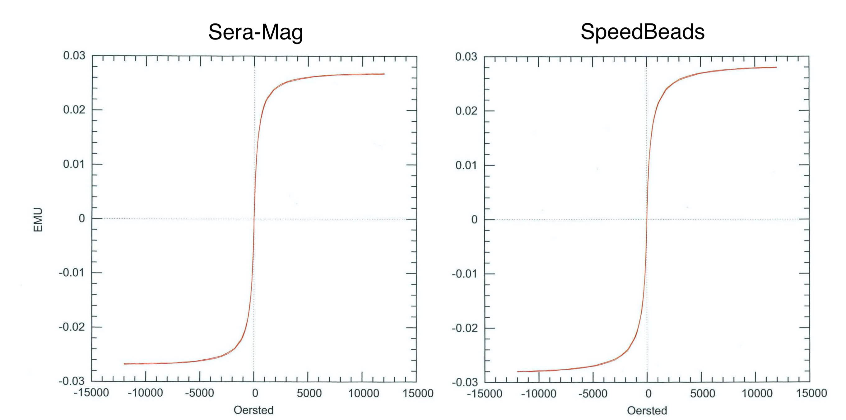
For an example, let’s use the datasheet for Sera-Mag and SpeedBead particles - two kinds of superparamagnetic nanoparticles manufactured by Sigma-Aldrich. The datasheet isn’t publicly available, but we got a hold of it by emailing our customer service representative.
The first page contains the following information:
| Property | Sera-Mag | SpeedBeads |
|---|---|---|
| Diameter (um) | 0.74 | 0.89 |
| Response Time (s) | 88 | 48 |
| Saturation (emu/g) | 27.1 | 44.4 |
| Surface Area (m2/g) | 49 | 64 |
| Density (g/cm3) | 2.22 | 2.83 |
The diameter / surface area can be used to approximate the volume term in our equation. Since we also have the density, we can compute the particle mass. This will be useful to plug into the particle tracing module / kinematics equations.
The datasheet also includes the response time, which is probably a measurement of the relaxation time. I asked the customer service representatives at Sigma-Aldrich but we couldn’t get a clear answer. It’s certainly the correct order of magnitude for magnetite at room temperature (see this study). It is also low enough to satisfy the “fast response” assumptions of our model.1 However, I would be wary about doing simulations that depend strongly on the response time, such as high-frequency magnetic fields, without knowing exactly how Sigma-Aldrich measured this value.
Hysteresis curves
The second page contains hysteresis curves for the Sera-Mag particles and the SpeedBeads that were obtained from Arkival Magnetics (a material testing lab) using a vibrating sample magnetometer. There’s also a table containing more magnetic properties.
| Property | Sera-Mag | SpeedBeads |
|---|---|---|
| Sigma | 27.1 | 44.4 |
| Hmax | 1.2e4 | 1.2e4 |
| Is | 2.683e-2 | 2.803e-2 |
| Ir | 4.191e-4 | -1.509e-4 |
| SQ | 1.562e-2 | -5.382e-3 |
| Mass | 9.9e-4 | 6.3e-4 |
| Hc | 4.653 | 9.426e-1 |
| dH | 4.165 | -1.356 |
| SFD | 8.951e-1 | -1.439 |
The datasheet doesn’t provide descriptions or units for most of the properties. However, it’s not too difficult to figure out what they mean.
Sigma is the saturation magnetization, expressed as emu/g, and Hmax is the largest field that was applied to the beads during testing. The dH parameter is most likely the increment by which the applied magnetic field was increased and decreased during testing.
Hc is the coercivity, or the magnetic field strength required to de-magnetize the material. Since superparamagnetic beads do not retain a strong remnant magnetic moment when the external field is turned off, Hc is very small.
Is and Ir refer to the saturation and residual magnetization, in emu units. This is a little tricky to figure out, since the usual names for the parameters would be Ms and Mr. However, their meaning becomes clear once we observe that the Is values are the same as the saturation magnetization on the B/H plots.
SQ and SFD are the squareness and switching field distribution parameters, respectively. These parameters describe the shape of the hysteresis loop, but they aren’t important for our model.
Getting parameters from the datasheet
Since we have the B-H curve, it’s easy to get the volume susceptibility. I used the web plot digitizer to get the data points from the graph, then fit a line to the region surrounding zero. The slope of this line is the magnetic susceptibility. The only tricky part is that the (unitless) susceptibility is actually different in the SI and CGS systems. To get the correct value in the SI system, we need to multiply by \(4\pi\).
Model files
For full reproducibility, here is a link the COMSOL files that were used for the blog post and for our paper on magnetic grids. The directory contains two files. One is the full simulation (magnetic fields and particle trajectories) for the simulations in my previous blog post. This uses the SpeedBeads and the D4X0-N52 magnet from K&J. The other file is a more complicated simulation involving grids of magnets that induce the interference pattern. It was used to generate the image at the top of this post.
Citation
If you found this post helpful for academic research, please consider citing the following papers. Also, feel free to get in touch - especially if you have questions or ended up using our methods!
[1] Coarsey, Chad, et al. “Development of a flow-free magnetic actuation platform for an automated microfluidic ELISA.” RSC advances 9.15 (2019): 8159-8168.
[2] Huang, Yangkun, et al. “Encoding Coacervate Droplets with Paramagnetism for Dynamical Reconfigurability and Spatial Addressability.” ACS nano 17.7 (2023): 6234-6246.
Notes
-
The error between the applied field and the magnetic moment decays exponentially with time. If full alignment takes 48 seconds, the magnetic moment will be mostly-aligned very quickly - fast enough for our simulations to be a good approximation. ↩